ordpy: A Python Package for Data Analysis with Permutation Entropy and Ordinal Network Methods
ordpy is a pure Python module [1] that implements data analysis methods based
on Bandt and Pompe’s [2] symbolic encoding scheme.
Note
If you have used ordpy in a scientific publication, we would appreciate
citations to the following reference [1]:
A. A. B. Pessa, H. V. Ribeiro, ordpy: A Python package for data analysis with permutation entropy and ordinal network methods, Chaos 31, 063110 (2021). arXiv:2102.06786
@misc{pessa2021ordpy,
  title         = {ordpy: A Python package for data analysis with permutation entropy and ordinal network methods},
  author        = {Arthur A. B. Pessa and Haroldo V. Ribeiro},
  journal       = {Chaos: An Interdisciplinary Journal of Nonlinear Science},
  volume        = {31},
  number        = {6},
  pages         = {063110},
  year          = {2021},
  doi           = {10.1063/5.0049901},
 }
ordpy implements the following data analysis methods:
Released on version 1.0.0 (February 2021):
Complexity-entropy plane for time series [4], [5] and images [3];
Multiscale complexity-entropy plane for time series [6] and images [7];
Tsallis [8] and Rényi [9] generalized complexity-entropy curves for time series and images;
Ordinal networks for time series [10], [11] and images [12];
Global node entropy of ordinal networks for time series [13], [11] and images [12].
Missing ordinal patterns [14] and missing transitions between ordinal patterns [11] for time series and images.
Released on version 1.1.0 (January 2023):
Weighted permutation entropy for time series [15] and images;
Fisher-Shannon plane for time series [16] and images;
Permutation Jensen-Shannon distance for time series [17] and images;
Four pattern permutation contrasts (up-down balance, persistence, rotational-asymmetry, and up-down scaling.) for time series [18];
Smoothness-structure plane for images [19].
Released on version 1.2.0 (April 2025):
Two-by-two ordinal patterns for images [21].
References
Installing
Ordpy can be installed via the command line using
pip install ordpy
or you can directly clone its git repository:
git clone https://github.com/arthurpessa/ordpy.git
cd ordpy
pip install -e .
Basic usage
We provide a notebook
illustrating how to use ordpy. This notebook reproduces all figures of our
article [1]. The code below shows simple applications of ordpy.
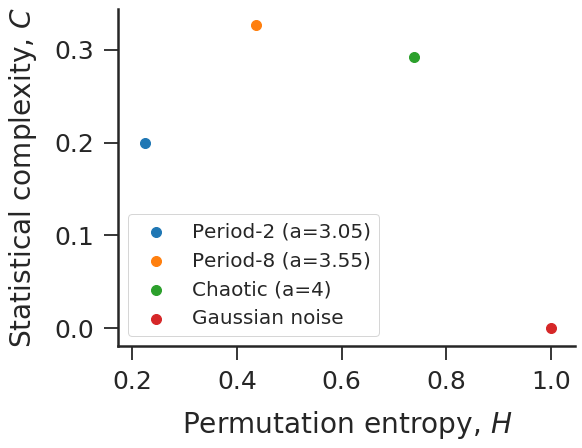
#Complexity-entropy plane for logistic map and Gaussian noise.

import numpy as np
import ordpy
from matplotlib import pylab as plt

def logistic(a=4, n=100000, x0=0.4):
    x = np.zeros(n)
    x[0] = x0
    for i in range(n-1):
        x[i+1] = a*x[i]*(1-x[i])
    return(x)

time_series = [logistic(a) for a in [3.05, 3.55, 4]]
time_series += [np.random.normal(size=100000)]

HC = [ordpy.complexity_entropy(series, dx=4) for series in time_series]


f, ax = plt.subplots(figsize=(8.19, 6.3))

for HC_, label_ in zip(HC, ['Period-2 (a=3.05)',
                            'Period-8 (a=3.55)',
                            'Chaotic (a=4)',
                            'Gaussian noise']):
    ax.scatter(*HC_, label=label_, s=100)

ax.set_xlabel('Permutation entropy, $H$')
ax.set_ylabel('Statistical complexity, $C$')

ax.legend()
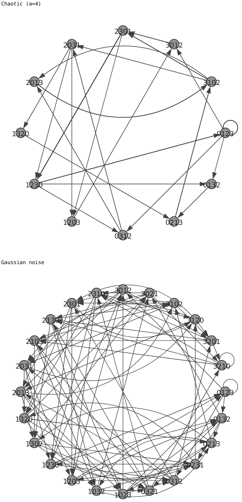
#Ordinal networks for logistic map and Gaussian noise.

import numpy as np
import igraph
import ordpy
from matplotlib import pylab as plt
from IPython.core.display import display, SVG

def logistic(a=4, n=100000, x0=0.4):
    x = np.zeros(n)
    x[0] = x0
    for i in range(n-1):
        x[i+1] = a*x[i]*(1-x[i])
    return(x)

time_series = [logistic(a=4), np.random.normal(size=100000)]

vertex_list, edge_list, edge_weight_list = list(), list(), list()
for series in time_series:
    v_, e_, w_   = ordpy.ordinal_network(series, dx=4)
    vertex_list += [v_]
    edge_list   += [e_]
    edge_weight_list += [w_]

def create_ig_graph(vertex_list, edge_list, edge_weight):

    G = igraph.Graph(directed=True)

    for v_ in vertex_list:
        G.add_vertex(v_)

    for [in_, out_], weight_ in zip(edge_list, edge_weight):
        G.add_edge(in_, out_, weight=weight_)

    return G

graphs = []

for v_, e_, w_ in zip(vertex_list, edge_list, edge_weight_list):
    graphs += [create_ig_graph(v_, e_, w_)]

def igplot(g):
    f = igraph.plot(g,
                    layout=g.layout_circle(),
                    bbox=(500,500),
                    margin=(40, 40, 40, 40),
                    vertex_label = [s.replace('|','') for s in g.vs['name']],
                    vertex_label_color='#202020',
                    vertex_color='#969696',
                    vertex_size=20,
                    vertex_font_size=6,
                    edge_width=(1 + 8*np.asarray(g.es['weight'])).tolist(),
                   )
    return f

for graph_, label_ in zip(graphs, ['Chaotic (a=4)',
                                   'Gaussian noise']):
    print(label_)
    display(SVG(igplot(graph_)._repr_svg_()))
List of functions
- ordpy.complexity_entropy(data, dx=3, dy=1, taux=1, tauy=1, probs=False, tie_precision=None)[source]
Calculates permutation entropy[2] and statistical complexity[4],[5] using an ordinal distribution obtained from data.
- Parameters:
data (array) – Array object in the format \([x_{1}, x_{2}, x_{3}, \ldots ,x_{n}]\) or \([[x_{11}, x_{12}, x_{13}, \ldots, x_{1m}], \ldots, [x_{n1}, x_{n2}, x_{n3}, \ldots, x_{nm}]]\) or an ordinal probability distribution (such as the ones returned by
ordpy.ordinal_distribution()).dx (int) – Embedding dimension (horizontal axis) (default: 3).
dy (int) – Embedding dimension (vertical axis); it must be 1 for time series (default: 1).
taux (int) – Embedding delay (horizontal axis) (default: 1).
tauy (int) – Embedding delay (vertical axis) (default: 1).
probs (boolean) – If True, it assumes data is an ordinal probability distribution. If False, data is expected to be a one- or two-dimensional array (default: False).
tie_precision (None, int) – If not None, data is rounded with tie_precision decimal numbers (default: None).
- Returns:
Values of normalized permutation entropy and statistical complexity.
- Return type:
tuple
Examples
>>> complexity_entropy([4,7,9,10,6,11,3], dx=2)
(0.9182958340544894, 0.06112816548804511)
>>>
>>> p = ordinal_distribution([4,7,9,10,6,11,3], dx=2, return_missing=True)[1]
>>> complexity_entropy(p, dx=2, probs=True)
(0.9182958340544894, 0.06112816548804511)
>>>
>>> complexity_entropy([[1,2,1],[8,3,4],[6,7,5]], dx=2, dy=2)
(0.3271564379782973, 0.2701200547320647)
>>>
>>> complexity_entropy([1/3, 1/15, 4/15, 2/15, 1/5, 0], dx=3, probs=True)
(0.8314454838586238, 0.16576716623440763)
>>>
>>> complexity_entropy([[1,2,1,4],[8,3,4,5],[6,7,5,6]],dx=3, dy=2)
(0.21070701155008006, 0.20704765093242872)
- ordpy.fisher_shannon(data, dx=3, dy=1, taux=1, tauy=1, probs=False, tie_precision=None)[source]
Calculates permutation entropy[2] and Fisher information[16] using an ordinal distribution obtained from data.
- Parameters:
data (array) – Array object in the format \([x_{1}, x_{2}, x_{3}, \ldots ,x_{n}]\) or \([[x_{11}, x_{12}, x_{13}, \ldots, x_{1m}], \ldots, [x_{n1}, x_{n2}, x_{n3}, \ldots, x_{nm}]]\) or an ordinal probability distribution (such as the ones returned by
ordpy.ordinal_distribution()).dx (int) – Embedding dimension (horizontal axis) (default: 3).
dy (int) – Embedding dimension (vertical axis); it must be 1 for time series (default: 1).
taux (int) – Embedding delay (horizontal axis) (default: 1).
tauy (int) – Embedding delay (vertical axis) (default: 1).
probs (boolean) – If True, it assumes data is an ordinal probability distribution. If False, data is expected to be a one- or two-dimensional array (default: False).
tie_precision (None, int) – If not None, data is rounded with tie_precision decimal numbers (default: None).
- Returns:
Values of normalized permutation entropy and Fisher information.
- Return type:
tuple
Examples
>>> fisher_shannon([4,7,9,10,6,11,3], dx=2)
(0.9182958340544896, 0.028595479208968325)
>>>
>>> p = ordinal_distribution([4,7,9,10,6,11,3], dx=2, return_missing=True)[1]
>>> fisher_shannon(p, dx=2, probs=True)
(0.9182958340544896, 0.028595479208968325)
>>>
>>> fisher_shannon([[1,2,1],[8,3,4],[6,7,5]], dx=2, dy=2)
(0.32715643797829735, 1.0)
>>>
>>> fisher_shannon([1/3, 1/15, 2/15, 3/15, 4/15, 0], dx=3, probs=True)
(0.8314454838586239, 0.19574180681374548)
>>>
>>> fisher_shannon([[1,2,1,4],[8,3,4,5],[6,7,5,6]], dx=3, dy=2)
(0.2107070115500801, 1.0)
- ordpy.global_node_entropy(data, dx=3, dy=1, taux=1, tauy=1, overlapping=True, connections='all', tie_precision=None)[source]
Calculates global node entropy[11],[13] for an ordinal network obtained from data. (Assumes directed and weighted edges).
- Parameters:
data (array, return of
ordpy.ordinal_network()) – Array object in the format \([x_{1}, x_{2}, x_{3}, \ldots ,x_{n}]\) or \([[x_{11}, x_{12}, x_{13}, \ldots, x_{1m}], \ldots, [x_{n1}, x_{n2}, x_{n3}, \ldots, x_{nm}]]\) or an ordinal network returned byordpy.ordinal_network()[*].dx (int) – Embedding dimension (horizontal axis) (default: 3).
dy (int) – Embedding dimension (vertical axis); it must be 1 for time series (default: 1).
taux (int) – Embedding delay (horizontal axis) (default: 1).
tauy (int) – Embedding delay (vertical axis) (default: 1).
overlapping (boolean) – If True, data is partitioned into overlapping sliding windows (default: True). If False, adjacent partitions are non-overlapping.
connections (str) – The ordinal network is constructed using ‘all’ permutation successions in a symbolic sequence or only ‘horizontal’ or ‘vertical’ successions. Parameter only valid for image data (default: ‘all’).
tie_precision (None, int) – If not None, data is rounded with tie_precision decimal numbers (default: None).
- Returns:
Value of global node entropy.
- Return type:
float
Notes
Examples
>>> global_node_entropy([1,2,3,4,5,6,7,8,9], dx=2)
0.0
>>>
>>> global_node_entropy(ordinal_network([1,2,3,4,5,6,7,8,9], dx=2))
0.0
>>>
>>> global_node_entropy(np.random.uniform(size=100000), dx=3)
1.4988332319747597
>>>
>>> global_node_entropy(random_ordinal_network(dx=3))
1.5
>>>
>>> global_node_entropy([[1,2,1,4],[8,3,4,5],[6,7,5,6]], dx=2, dy=2, connections='horizontal')
0.25
>>>
>>> global_node_entropy([[1,2,1,4],[8,3,4,5],[6,7,5,6]], dx=2, dy=2, connections='vertical')
0.0
- ordpy.logq(x, q=1)[source]
Calculates the q-logarithm of x.
- Parameters:
x (float, array) – Real number or array containing real numbers.
q (float) – Tsallis’s q parameter (default: 1).
- Returns:
Value or array of values containing the q-logarithm of x.
- Return type:
float or array
Notes
The q-logarithm of x is defined as[†]
\[\]log_q (x) = frac{x^{1-q} - 1}{1-q}~~text{for}~~qneq 1
and \(\log_q (x) = \log (x)\) for \(q=1\).
Examples
>>> logq(np.math.e)
1.0
>>>
>>> logq([np.math.e for i in range(5)])
array([1., 1., 1., 1., 1.])
- ordpy.maximum_complexity_entropy(dx=3, dy=1, m=1)[source]
Generates data corresponding to values of normalized permutation entropy and statistical complexity which delimit the upper boundary in the complexity-entropy causality plane[20],[‡].
- Parameters:
dx (int) – Embedding dimension (horizontal axis) (default: 3).
dy (int) – Embedding dimension (vertical axis); must be 1 for time series (default: 1).
m (int) – The length of the returned array containing values of permutation entropy and statistical complexity is given by \([(d_x \times d_y)!-1] \times m\).
- Returns:
Values of normalized permutation entropy and statistical complexity belonging to the upper limiting curve of the complexity-entropy causality plane.
- Return type:
array
Notes
Examples
>>> maximum_complexity_entropy(dx=3, dy=1, m=1)
array([[-0.        , -0.        ],
       [ 0.38685281,  0.27123863],
       [ 0.61314719,  0.29145164],
       [ 0.77370561,  0.22551573],
       [ 0.8982444 ,  0.12181148]])
>>>
>>> maximum_complexity_entropy(dx=3, dy=1, m=2)
array([[-0.        , -0.        ],
       [ 0.251463  ,  0.19519391],
       [ 0.38685281,  0.27123863],
       [ 0.57384034,  0.28903864],
       [ 0.61314719,  0.29145164],
       [ 0.76241899,  0.2294088 ],
       [ 0.77370561,  0.22551573],
       [ 0.89621768,  0.12320718],
       [ 0.8982444 ,  0.12181148],
       [ 1.        ,  0.        ]])
- ordpy.minimum_complexity_entropy(dx=3, dy=1, size=100)[source]
Generates data corresponding to values of normalized permutation entropy and statistical complexity which delimit the lower boundary in the complexity-entropy causality plane[20],[§].
- Parameters:
dx (int) – Embedding dimension (horizontal axis) (default: 3).
dy (int) – Embedding dimension (vertical axis); must be 1 for time series (default: 1).
size (int) – The length of the array returned containing pairs of values of permutation entropy and statistical complexity.
- Returns:
Values of normalized permutation entropy and statistical complexity belonging to the lower limiting curve of the complexity-entropy causality plane.
- Return type:
array
Notes
Examples
>>> minimum_complexity_entropy(dx=3, size=10)
array([[-0.        , -0.        ],
       [ 0.25534537,  0.17487933],
       [ 0.43376898,  0.21798915],
       [ 0.57926767,  0.21217508],
       [ 0.70056313,  0.18118876],
       [ 0.80117413,  0.1378572 ],
       [ 0.88242522,  0.09085847],
       [ 0.94417789,  0.04723328],
       [ 0.98476216,  0.01396083],
       [ 1.        ,  0.        ]])
>>>
>>> minimum_complexity_entropy(dx=4, size=5)
array([[-0.00000000e+00, -0.00000000e+00],
       [ 4.09625322e-01,  2.10690777e-01],
       [ 6.90580872e-01,  1.84011590e-01],
       [ 8.96072453e-01,  8.64190054e-02],
       [ 1.00000000e+00, -3.66606083e-16]])
- ordpy.missing_links(data, dx=3, dy=1, return_fraction=True, return_missing=True, tie_precision=None)[source]
Identifies transitions between ordinal patterns (permutations) not occurring in data. (These transtitions correspond to directed edges in ordinal networks[11].) Assumes overlapping windows and unitary embedding delay. In case dx>1 and dy>1, both ‘horizontal’ and ‘vertical’ connections are considered (see
ordpy.ordinal_network()).- Parameters:
data (array, return of
ordpy.ordinal_network()) – Array object in the format \([x_{1}, x_{2}, x_{3}, \ldots ,x_{n}]\) or \([[x_{11}, x_{12}, x_{13}, \ldots, x_{1m}], \ldots, [x_{n1}, x_{n2}, x_{n3}, \ldots, x_{nm}]]\) or the nodes, edges and edge weights returned byordpy.ordinal_network().dx (int) – Embedding dimension (horizontal axis) (default: 3)
dy (int) – Embedding dimension (vertical axis); must be 1 for time series (default: 1).
return_fraction (boolean) – if True, returns the fraction of missing links among ordinal patterns relative to the total number of possible links (transitions) for given values of dx and dy (default: True). If False, returns the raw number of missing links.
return_missing (boolean) – if True, returns the missing links in data; if False, it only returns the fraction/number of these missing links.
tie_precision (None, int) – If not None, data is rounded with tie_precision decimal numbers (default: None).
- Returns:
Tuple containing an array and a float indicating missing links and their relative fraction (or raw number).
- Return type:
tuple
Examples
>>> missing_links([4,7,9,10,6,11,3], dx=2, return_fraction=False)
(array([['1|0', '1|0']], dtype='<U3'), 1)
>>>
>>> missing_links(ordinal_network([4,7,9,10,6,11,3], dx=2), dx=2, return_fraction=True)
(array([['1|0', '1|0']], dtype='<U3'), 0.25)
>>>
>>> missing_links([4,7,9,10,6,11,3,5,6,2,3,1], dx=3, return_fraction=False)
(array([['0|1|2', '0|2|1'],
        ['0|2|1', '1|0|2'],
        ['0|2|1', '1|2|0'],
        ['0|2|1', '2|1|0'],
        ['1|0|2', '0|1|2'],
        ['1|0|2', '0|2|1'],
        ['1|2|0', '0|2|1'],
        ['2|0|1', '2|1|0'],
        ['2|1|0', '1|0|2'],
        ['2|1|0', '1|2|0'],
        ['2|1|0', '2|1|0']], dtype='<U5'), 11)
- ordpy.missing_patterns(data, dx=3, dy=1, taux=1, tauy=1, return_fraction=True, return_missing=True, probs=False, tie_precision=None)[source]
Identifies ordinal patterns (permutations) not occurring in data[14].
- Parameters:
data (array, return of
ordpy.ordinal_distribution()) – Array object in the format \([x_{1}, x_{2}, x_{3}, \ldots ,x_{n}]\) or \([[x_{11}, x_{12}, x_{13}, \ldots, x_{1m}], \ldots, [x_{n1}, x_{n2}, x_{n3}, \ldots, x_{nm}]]\) or the ordinal patterns and probabilities returned byordpy.ordinal_distribution()with return_missing=True.dx (int) – Embedding dimension (horizontal axis) (default: 3).
dy (int) – Embedding dimension (vertical axis); must be 1 for time series (default: 1).
taux (int) – Embedding delay (horizontal axis) (default: 1).
tauy (int) – Embedding delay (vertical axis) (default: 1).
return_fraction (boolean) – if True, returns the fraction of missing ordinal patterns relative to the total number of ordinal patterns for given values of dx and dy (default: True); if False, returns the raw number of missing patterns.
return_missing (boolean) – if True, returns the missing ordinal patterns in data (default: True); if False, it only returns the fraction/number of these missing patterns.
probs (boolean) – If True, assumes data to be the return of
ordpy.ordinal_distribution()with return_missing=True. If False, data is expected to be a one- or two-dimensional array (default: False).tie_precision (None, int) – If not None, data is rounded with tie_precision decimal numbers (default: None).
- Returns:
Tuple containing an array and a float indicating missing ordinal patterns and their relative fraction (or raw number).
- Return type:
tuple
Examples
>>> missing_patterns([4,7,9,10,6,11,3], dx=2, return_fraction=False)
(array([], shape=(0, 2), dtype=int64), 0)
>>>
>>> missing_patterns([4,7,9,10,6,11,3,5,6,2,3,1], dx=3, return_fraction=True, return_missing=False)
0.3333333333333333
>>>
>>> missing_patterns(ordinal_distribution([4,7,9,10,6,11,3], dx=2, return_missing=True), dx=2, probs=True)
(array([], shape=(0, 2), dtype=int64), 0.0)
>>>
>>> missing_patterns(ordinal_distribution([4,7,9,10,6,11,3], dx=3, return_missing=True), dx=3, probs=True)
(array([[0, 2, 1],
        [1, 2, 0],
        [2, 1, 0]]), 0.5)
- ordpy.ordinal_distribution(data, dx=3, dy=1, taux=1, tauy=1, return_missing=False, tie_precision=None, ordered=False)[source]
Applies the Bandt and Pompe[2] symbolization approach to obtain a probability distribution of ordinal patterns (permutations) from data.
- Parameters:
data (array) – Array object in the format \([x_{1}, x_{2}, x_{3}, \ldots ,x_{n}]\) or \([[x_{11}, x_{12}, x_{13}, \ldots, x_{1m}], \ldots, [x_{n1}, x_{n2}, x_{n3}, \ldots, x_{nm}]]\).
dx (int) – Embedding dimension (horizontal axis) (default: 3).
dy (int) – Embedding dimension (vertical axis); it must be 1 for time series (default: 1).
taux (int) – Embedding delay (horizontal axis) (default: 1).
tauy (int) – Embedding delay (vertical axis) (default: 1).
return_missing (boolean) – If True, it returns ordinal patterns not appearing in the symbolic sequence obtained from data. If False, these missing patterns (permutations) are omitted (default: False).
tie_precision (None, int) – If not None, data is rounded with tie_precision decimal numbers (default: None).
ordered (boolean) – If True, it also returns ordinal patterns not appearing in the symbolic sequence obtained from data in ascending ordered. The return_missing parameter must also be True.
- Returns:
Tuple containing two arrays, one with the ordinal patterns and another with their corresponding probabilities.
- Return type:
tuple
Examples
>>> ordinal_distribution([4,7,9,10,6,11,3], dx=2)
(array([[0, 1],
        [1, 0]]),
 array([0.66666667, 0.33333333]))
>>>
>>> ordinal_distribution([4,7,9,10,6,11,3], dx=3, return_missing=True)
(array([[0, 1, 2],
        [1, 0, 2],
        [2, 0, 1],
        [0, 2, 1],
        [1, 2, 0],
        [2, 1, 0]]),
 array([0.4, 0.2, 0.4, 0. , 0. , 0. ]))
>>>
>>> ordinal_distribution([[1,2,1],[8,3,4],[6,7,5]], dx=2, dy=2)
(array([[0, 1, 3, 2],
        [1, 0, 2, 3],
        [1, 2, 3, 0]]),
 array([0.5 , 0.25, 0.25]))
>>>
>>> ordinal_distribution([[1,2,1,4],[8,3,4,5],[6,7,5,6]], dx=2, dy=2, taux=2)
(array([[0, 1, 3, 2],
        [0, 2, 1, 3],
        [1, 3, 2, 0]]),
 array([0.5 , 0.25, 0.25]))
- ordpy.ordinal_network(data, dx=3, dy=1, taux=1, tauy=1, normalized=True, overlapping=True, directed=True, connections='all', tie_precision=None)[source]
Maps a data set into the elements (nodes, edges and edge weights) of its corresponding ordinal network representation[10],[11],[12].
- Parameters:
data (array) – Array object in the format \([x_{1}, x_{2}, x_{3}, \ldots ,x_{n}]\) or \([[x_{11}, x_{12}, x_{13}, \ldots, x_{1m}], \ldots, [x_{n1}, x_{n2}, x_{n3}, \ldots, x_{nm}]]\).
dx (int) – Embedding dimension (horizontal axis) (default: 3).
dy (int) – Embedding dimension (vertical axis); it must be 1 for time series (default: 1).
taux (int) – Embedding delay (horizontal axis) (default: 1).
tauy (int) – Embedding delay (vertical axis) (default: 1).
normalized (boolean) – If True, edge weights represent transition probabilities between permutations (default: True). If False, edge weights are transition counts.
overlapping (boolean) – If True, data is partitioned into overlapping sliding windows (default: True). If False, adjacent partitions are non-overlapping.
directed (boolean) – If True, ordinal network edges are directed (default: True). If False, edges are undirected.
connections (str) – The ordinal network is constructed using ‘all’ permutation successions in a symbolic sequence or only ‘horizontal’ or ‘vertical’ successions. Parameter only valid for image data (default: ‘all’).
tie_precision (None, int) – If not None, data is rounded with tie_precision decimal numbers (default: None).
- Returns:
Tuple containing three arrays corresponding to nodes, edges and edge weights of an ordinal network.
- Return type:
tuple
Examples
>>> ordinal_network([4,7,9,10,6,11,8,3,7], dx=2, normalized=False)
(array(['0|1', '1|0'], dtype='<U3'),
 array([['0|1', '0|1'],
        ['0|1', '1|0'],
        ['1|0', '0|1'],
        ['1|0', '1|0']], dtype='<U3'),
 array([2, 2, 2, 1]))
>>>
>>> ordinal_network([4,7,9,10,6,11,8,3,7], dx=2, overlapping=False, normalized=False)
(array(['0|1', '1|0'], dtype='<U3'),
 array([['0|1', '0|1'],
        ['0|1', '1|0']], dtype='<U3'),
 array([2, 1]))
>>>
>>> ordinal_network([[1,2,1],[8,3,4],[6,7,5]], dx=2, dy=2, normalized=False)
(array(['0|1|3|2', '1|0|2|3', '1|2|3|0'], dtype='<U7'),
 array([['0|1|3|2', '1|0|2|3'],
        ['0|1|3|2', '1|2|3|0'],
        ['1|0|2|3', '0|1|3|2'],
        ['1|2|3|0', '0|1|3|2']], dtype='<U7'),
 array([1, 1, 1, 1]))
>>>
>>> ordinal_network([[1,2,1],[8,3,4],[6,7,5]], dx=2, dy=2, normalized=True, connections='horizontal')
(array(['0|1|3|2', '1|0|2|3', '1|2|3|0'], dtype='<U7'),
 array([['0|1|3|2', '1|0|2|3'],
        ['1|2|3|0', '0|1|3|2']], dtype='<U7'),
 array([0.5, 0.5]))
- ordpy.ordinal_sequence(data, dx=3, dy=1, taux=1, tauy=1, overlapping=True, tie_precision=None)[source]
Applies the Bandt and Pompe[2] symbolization approach to obtain a sequence of ordinal patterns (permutations) from data.
- Parameters:
data (array) – Array object in the format \([x_{1}, x_{2}, x_{3}, \ldots ,x_{n}]\) or \([[x_{11}, x_{12}, x_{13}, \ldots, x_{1m}], \ldots, [x_{n1}, x_{n2}, x_{n3}, \ldots, x_{nm}]]\) (\(n \times m\)).
dx (int) – Embedding dimension (horizontal axis) (default: 3).
dy (int) – Embedding dimension (vertical axis); it must be 1 for time series (default: 1).
taux (int) – Embedding delay (horizontal axis) (default: 1).
tauy (int) – Embedding delay (vertical axis) (default: 1).
overlapping (boolean) – If True, data is partitioned into overlapping sliding windows (default: True). If False, adjacent partitions are non-overlapping.
tie_precision (None, int) – If not None, data is rounded with tie_precision number of decimals (default: None).
- Returns:
Array containing the sequence of ordinal patterns.
- Return type:
array
Examples
>>> ordinal_sequence([4,7,9,10,6,11,3], dx=2)
array([[0, 1],
       [0, 1],
       [0, 1],
       [1, 0],
       [0, 1],
       [1, 0]])
>>>
>>> ordinal_sequence([4,7,9,10,6,11,3], dx=2, taux=2)
array([[0, 1],
       [0, 1],
       [1, 0],
       [0, 1],
       [1, 0]])
>>>
>>> ordinal_sequence([[1,2,1,4],[8,3,4,5],[6,7,5,6]], dx=2, dy=2)
array([[[0, 1, 3, 2],
        [1, 0, 2, 3],
        [0, 1, 2, 3]],
       [[1, 2, 3, 0],
        [0, 1, 3, 2],
        [0, 1, 2, 3]]])
>>>
>>> ordinal_sequence([1.3, 1.2], dx=2), ordinal_sequence([1.3, 1.2], dx=2, tie_precision=0)
(array([[1, 0]]), array([[0, 1]]))
- ordpy.permutation_contrasts(data, taux=1, tie_precision=None)[source]
Calculates the four pattern (permutation) contrasts [18] of a time series (with dx=3) using an ordinal distribution obtained from data.
- Parameters:
data (array) – Array object containing a pair of arrays in the format \([x_{1}, x_{2}, x_{3}, \ldots ,x_{n}]\).
taux (int) – Embedding delay (horizontal axis) (default: 1).
tie_precision (None, int) – If not None, data is rounded with tie_precision decimal numbers (default: None).
- Returns:
Tuple containing values corresponding to the pattern (permutation) contrasts: up-down balance, persistence, rotational-asymmetry, and up-down scaling.
- Return type:
tuple
Examples
>>> permutation_contrasts([4,7,9,10,6,11,3])
(0.4, 0.4, 0.6, -0.2)
>>>
>>> permutation_contrasts([4,7,9,10,6,11,3], taux=2)
(0.0, 0.666, -0.333, 0.333)
>>>
>>> permutation_contrasts([5,2,3,4,2,7,4])
(0.2, 0.2, 0.0, 0.0)
>>>
>>> permutation_contrasts([5, 2, 3, 4, 2, 7, 4], taux=2)
(0.0, 0.666, 0.333, 0.333)
- ordpy.permutation_entropy(data, dx=3, dy=1, taux=1, tauy=1, base='e', normalized=True, probs=False, tie_precision=None)[source]
Calculates the Shannon entropy using an ordinal distribution obtained from data[2],[3].
- Parameters:
data (array) – Array object in the format \([x_{1}, x_{2}, x_{3}, \ldots ,x_{n}]\) or \([[x_{11}, x_{12}, x_{13}, \ldots, x_{1m}], \ldots, [x_{n1}, x_{n2}, x_{n3}, \ldots, x_{nm}]]\) or an ordinal probability distribution (such as the ones returned by
ordpy.ordinal_distribution()).dx (int) – Embedding dimension (horizontal axis) (default: 3).
dy (int) – Embedding dimension (vertical axis); it must be 1 for time series (default: 1).
taux (int) – Embedding delay (horizontal axis) (default: 1).
tauy (int) – Embedding delay (vertical axis) (default: 1).
base (str, int) – Logarithm base in Shannon’s entropy. Either ‘e’ or 2 (default: ‘e’).
normalized (boolean) – If True, permutation entropy is normalized by its maximum value (default: True). If False, it is not.
probs (boolean) – If True, it assumes data is an ordinal probability distribution. If False, data is expected to be a one- or two-dimensional array (default: False).
tie_precision (None, int) – If not None, data is rounded with tie_precision decimal numbers (default: None).
- Returns:
Value of permutation entropy.
- Return type:
float
Examples
>>> permutation_entropy([4,7,9,10,6,11,3], dx=2, base=2, normalized=True)
0.9182958340544896
>>>
>>> permutation_entropy([.5,.5], dx=2, base=2, normalized=False, probs=True)
1.0
>>>
>>> permutation_entropy([[1,2,1],[8,3,4],[6,7,5]], dx=2, dy=2, base=2, normalized=True)
0.32715643797829735
>>>
>>> permutation_entropy([[1,2,1,4],[8,3,4,5],[6,7,5,6]], dx=2, dy=2, taux=2, base='e', normalized=False)
1.0397207708399179
- ordpy.permutation_js_distance(data, dx=3, dy=1, taux=1, tauy=1, base='e', normalized=True, tie_precision=None)[source]
Calculates the permutation Jensen-Shannon distance[17] between multiple time series (or channels of a multivariate time series) or multiple matrices (images) using ordinal distributions obtained from data.
- Parameters:
data (array) – Array object containing arrays in the format \([x_{1}, x_{2}, x_{3}, \ldots ,x_{n}]\) or \([[x_{11}, x_{12}, x_{13}, \ldots, x_{1m}], \ldots, [x_{n1}, x_{n2}, x_{n3}, \ldots, x_{nm}]]\).
dx (int) – Embedding dimension (horizontal axis) (default: 3).
dy (int) – Embedding dimension (vertical axis); it must be 1 for time series (default: 1).
taux (int) – Embedding delay (horizontal axis) (default: 1).
tauy (int) – Embedding delay (vertical axis) (default: 1).
base (str, int) – Logarithm base in Shannon’s entropy. Either ‘e’ or 2 (default: ‘e’).
normalized (boolean) – If True, the permutation Jensen-Shannon distance is normalized by the logarithm of 2. (default: True). If False, it is not.
tie_precision (None, int) – If not None, data is rounded with tie_precision decimal numbers (default: None).
- Returns:
Value of permutation Jensen-Shannon distance.
- Return type:
float
Examples
>>> permutation_js_distance([[1,2,6,5,4], [1,2,1]], dx=3, base=2, normalized=False)
0.677604543245723
>>>
>>> permutation_js_distance([[1,2,6,5,4], [1,2,1]], dx=3, base='e', normalized=False)
0.5641427870206323
>>>
>>> permutation_js_distance([[[1,2,6],[4,2,6]], [[1,2,6],[1,2,4]]], dx=2, dy=2)
0.7071067811865476
>>>
>>> permutation_js_distance([[[1,2,6,5,4],[4,2,6,3,4]], [[1,2,6],[1,2,4]]], dx=2, dy=2)
0.809715420521041
- ordpy.random_ordinal_network(dx=3, dy=1, overlapping=True)[source]
Generates the nodes, edges and edge weights of a random ordinal network: the theoretically expected network representation of a random time series[11] or a random two-dimensional array[12]. (Assumes directed edges and unitary embedding delays.)
- Parameters:
dx (int) – Embedding dimension (horizontal axis) (default: 3).
dy (int) – Embedding dimension (vertical axis); it must be 1 for time series (default: 1).
overlapping (boolean) – If True, data is partitioned into overlapping sliding windows (default: True). If False, adjacent partitions are non-overlapping.
- Returns:
Tuple containing three arrays corresponding to nodes, edges and edge weights of the random ordinal network.
- Return type:
tuple
Examples
>>> random_ordinal_network(dx=2)
(array(['0|1', '1|0'], dtype='<U3'),
 array([['0|1', '0|1'],
        ['0|1', '1|0'],
        ['1|0', '0|1'],
        ['1|0', '1|0']], dtype='<U3'),
 array([0.16666667, 0.33333333, 0.33333333, 0.16666667]))
>>>
>>> random_ordinal_network(dx=2, overlapping=False)
(array(['0|1', '1|0'], dtype='<U3'),
 array([['0|1', '0|1'],
        ['0|1', '1|0'],
        ['1|0', '0|1'],
        ['1|0', '1|0']], dtype='<U3'),
 array([0.25, 0.25, 0.25, 0.25]))
- ordpy.renyi_complexity_entropy(data, alpha=1, dx=3, dy=1, taux=1, tauy=1, probs=False, tie_precision=None)[source]
Calculates the Rényi normalized permutation entropy and statistical complexity[9] using an ordinal distribution obtained from data.
- Parameters:
data (array) – Array object in the format \([x_{1}, x_{2}, x_{3}, \ldots ,x_{n}]\) or \([[x_{11}, x_{12}, x_{13}, \ldots, x_{1m}], \ldots, [x_{n1}, x_{n2}, x_{n3}, \ldots, x_{nm}]]\) or an ordinal probability distribution (such as the ones returned by
ordpy.ordinal_distribution()).alpha (float, array) – Rényi’s alpha parameter (default: 1); an array of values is also accepted for this parameter.
dx (int) – Embedding dimension (horizontal axis) (default: 3).
dy (int) – Embedding dimension (vertical axis); it must be 1 for time series (default: 1).
taux (int) – Embedding delay (horizontal axis) (default: 1).
tauy (int) – Embedding delay (vertical axis) (default: 1).
probs (boolean) – If True, it assumes data is an ordinal probability distribution. If False, data is expected to be a one- or two-dimensional array (default: False).
tie_precision (None, int) – If not None, data is rounded with tie_precision decimal numbers (default: None).
- Returns:
Value(s) of normalized permutation entropy and statistical complexity in Rényi’s formalism.
- Return type:
array
Examples
>>> renyi_complexity_entropy([4,7,9,10,6,11,3], dx=2)
array([0.91829583, 0.06112817])
>>>
>>> p = ordinal_distribution([4,7,9,10,6,11,3], dx=2, return_missing=True)[1]
>>> renyi_complexity_entropy(p, dx=2, probs=True)
array([0.91829583, 0.06112817])
>>>
>>> renyi_complexity_entropy([4,7,9,10,6,11,3], alpha=2, dx=2)
array([0.84799691, 0.08303895])
>>>
>>> renyi_complexity_entropy([1/3, 1/15, 4/15, 2/15, 1/5, 0], dx=3, probs=True)
array([0.83144548, 0.16576717])
>>>
>>> renyi_complexity_entropy([4,7,9,10,6,11,3], alpha=[1, 2], dx=2)
array([[0.91829583, 0.06112817],
       [0.84799691, 0.08303895]])
>>>
>>> renyi_complexity_entropy([[1,2,1,4],[8,3,4,5],[6,7,5,6]], alpha=3, dx=3, dy=2)
array([0.21070701, 0.20975673])
- ordpy.renyi_entropy(data, alpha=1, dx=3, dy=1, taux=1, tauy=1, probs=False, tie_precision=None)[source]
Calculates the normalized Rényi permutation entropy[9] using an ordinal distribution obtained from data.
- Parameters:
data (array) –
- Array object in the format \([x_{1}, x_{2}, x_{3}, \ldots ,x_{n}]\)
or \([[x_{11}, x_{12}, x_{13}, \ldots, x_{1m}], \ldots, [x_{n1}, x_{n2}, x_{n3}, \ldots, x_{nm}]]\) or an ordinal probability distribution (such as the ones returned by
alpha (float, array) – Rényi’s alpha parameter (default: 1); an array of values is also accepted for this parameter.
dx (int) – Embedding dimension (horizontal axis) (default: 3).
dy (int) – Embedding dimension (vertical axis); it must be 1 for time series (default: 1).
taux (int) – Embedding delay (horizontal axis) (default: 1).
tauy (int) – Embedding delay (vertical axis) (default: 1).
probs (boolean) – If True, it assumes data is an ordinal probability distribution. If False, data is expected to be a one- or two-dimensional array (default: False).
tie_precision (None, int) – If not None, data is rounded with tie_precision decimal numbers (default: None).
- Returns:
Value(s) of the normalized Rényi permutation entropy.
- Return type:
float, array
Examples
>>> renyi_entropy([4,7,9,10,6,11,3], dx=2)
0.9182958340544894
>>>
>>> renyi_entropy([4,7,9,10,6,11,3], alpha=2, dx=2)
0.84799690655495
>>>
>>> renyi_entropy([1/3, 1/15, 4/15, 2/15, 1/5, 0], dx=3, probs=True)
0.8314454838586238
>>>
>>> renyi_entropy([4,7,9,10,6,11,3], alpha=[1,2], dx=2)
array([0.91829583, 0.84799691])
>>>
>>> renyi_entropy([4,7,9,10,6,11,3], alpha=2, dx=3)
0.5701944178769374
- ordpy.smoothness_structure(data, taux=1, tauy=1, tie_precision=None)[source]
Calculates the smoothness and curve structure[19] of an image (with embedding parameters dx=dy=2) using an ordinal distribution obtained from data.
- Parameters:
data (array) – Array object in the format \([[x_{11}, x_{12}, x_{13}, \ldots, x_{1m}], \ldots, [x_{n1}, x_{n2}, x_{n3}, \ldots, x_{nm}]]\).
taux (int) – Embedding delay (horizontal axis) (default: 1).
tauy (int) – Embedding delay (vertical axis) (default: 1).
tie_precision (None, int) – If not None, data is rounded with tie_precision decimal numbers (default: None).
- Returns:
Values of smoothness and curve structure.
- Return type:
tuple
Examples
>>> smoothness_structure([[1,2,1,4],[8,3,4,5],[6,7,5,6]])
(0.0, 0.333)
>>>
>>> smoothness_structure([[1,2,1,4],[8,3,4,5],[6,7,5,6]], taux=2, tauy=1)
(-0.0833, 0.75)
>>>
>>> smoothness_structure([[1,2,1,4],[8,3,4,5],[6,7,5,6]], taux=2, tauy=2)
(-0.333, 1.0)
- ordpy.tsallis_complexity_entropy(data, q=1, dx=3, dy=1, taux=1, tauy=1, probs=False, tie_precision=None)[source]
Calculates the Tsallis normalized permutation entropy and statistical complexity[8] using an ordinal distribution obtained from data.
- Parameters:
data (array) –
- Array object in the format \([x_{1}, x_{2}, x_{3}, \ldots ,x_{n}]\)
or \([[x_{11}, x_{12}, x_{13}, \ldots, x_{1m}], \ldots, [x_{n1}, x_{n2}, x_{n3}, \ldots, x_{nm}]]\) or an ordinal probability distribution (such as the ones returned by
q (float, array) – Tsallis’s q parameter (default: 1); an array of values is also accepted for this parameter.
dx (int) – Embedding dimension (horizontal axis) (default: 3).
dy (int) – Embedding dimension (vertical axis); it must be 1 for time series (default: 1).
taux (int) – Embedding delay (horizontal axis) (default: 1).
tauy (int) – Embedding delay (vertical axis) (default: 1).
probs (boolean) – If True, it assumes data is an ordinal probability distribution. If False, data is expected to be a one- or two-dimensional array (default: False).
tie_precision (None, int) – If not None, data is rounded with tie_precision decimal numbers (default: None).
- Returns:
Value(s) of normalized permutation entropy and statistical complexity in Tsallis’s formalism.
- Return type:
array
Examples
>>> tsallis_complexity_entropy([4,7,9,10,6,11,3], dx=2)
array([0.91829583, 0.06112817])
>>>
>>> p = ordinal_distribution([4,7,9,10,6,11,3], dx=2, return_missing=True)[1]
>>> tsallis_complexity_entropy(p, dx=2, probs=True)
array([0.91829583, 0.06112817])
>>>
>>> tsallis_complexity_entropy([1/3, 1/15, 4/15, 2/15, 1/5, 0], dx=3, probs=True)
array([0.83144548, 0.16576717])
>>>
>>> tsallis_complexity_entropy([4,7,9,10,6,11,3], dx=2, q=[1,2])
array([[0.91829583, 0.06112817],
       [0.88888889, 0.07619048]])
>>>
>>> tsallis_complexity_entropy([4,7,9,10,6,11,3], q=2, dx=2)
array([0.88888889, 0.07619048])
>>>
>>> tsallis_complexity_entropy([[1,2,1,4],[8,3,4,5],[6,7,5,6]], q=3, dx=3, dy=2)
array([0.93750181, 0.92972165])
- ordpy.tsallis_entropy(data, q=1, dx=3, dy=1, taux=1, tauy=1, probs=False, tie_precision=None)[source]
Calculates the normalized Tsallis permutation entropy[8] using an ordinal distribution obtained from data.
- Parameters:
data (array) –
- Array object in the format \([x_{1}, x_{2}, x_{3}, \ldots ,x_{n}]\)
or \([[x_{11}, x_{12}, x_{13}, \ldots, x_{1m}], \ldots, [x_{n1}, x_{n2}, x_{n3}, \ldots, x_{nm}]]\) or an ordinal probability distribution (such as the ones returned by
q (float or array) – Tsallis’s q parameter (default: 1); an array of values is also accepted for this parameter.
dx (int) – Embedding dimension (horizontal axis) (default: 3).
dy (int) – Embedding dimension (vertical axis); it must be 1 for time series (default: 1).
taux (int) – Embedding delay (horizontal axis) (default: 1).
tauy (int) – Embedding delay (vertical axis) (default: 1).
probs (boolean) – If True, it assumes data is an ordinal probability distribution. If False, data is expected to be a one- or two-dimensional array (default: False).
tie_precision (None, int) – If not None, data is rounded with tie_precision decimal numbers (default: None).
- Returns:
Value(s) of the normalized Tsallis permutation entropy.
- Return type:
float, array
Examples
>>> tsallis_entropy([4,7,9,10,6,11,3], dx=2)
0.9182958340544894
>>>
>>> tsallis_entropy([4,7,9,10,6,11,3], q=[1,2], dx=2)
array([0.91829583, 0.88888889])
>>>
>>> tsallis_entropy([4,7,9,10,6,11,3], q=2, dx=2)
0.888888888888889
>>>
>>> tsallis_entropy([1/3, 1/15, 4/15, 2/15, 1/5, 0], dx=3, probs=True)
0.8314454838586238
>>>
>>> tsallis_entropy([4,7,9,10,6,11,3], q=2, dx=3)
0.768
- ordpy.two_by_two_patterns(data, taux=1, tauy=1, overlapping=True, tie_patterns=True, group_patterns=False, tie_precision=None)[source]
Extracts the distribution ordinal patterns from a two-dimensional array of data[21],[19].
- Parameters:
data (array) – Two dimensional array object in the format \([[x_{11}, x_{12}, x_{13}, \ldots, x_{1m}], \ldots, [x_{n1}, x_{n2}, x_{n3}, \ldots, x_{nm}]]\) (\(n \times m\)).
taux (int) – Embedding delay (horizontal axis) (default: 1).
tauy (int) – Embedding delay (vertical axis) (default: 1).
overlapping (boolean) – If True, data is partitioned into overlapping sliding windows (default: True). If False, adjacent partitions are non-overlapping.
tie_patterns (boolean) – If True, ties within partitions generate different ordinal patterns, yielding 75 unique ordinal patterns[21] (default: True). Otherwise, ties are ignored and only 24 unique ordinal patterns are generated[19].
group_patterns (boolean) – If True, the function returns a dictionary with the probabilities of each ordinal pattern grouped by their types (default: False). Otherwise, it returns a dictionary with the probabilities of all ordinal patterns. If tie_patterns is True, there are 11 groups of ordinal patterns named with letters from A to K. If tie_patterns is False, there are 3 groups of ordinal patterns named (I), (II) and (III).
tie_precision (None, int) – If not None, data is rounded with tie_precision number of decimals (default: None).
- Returns:
Dictionary with the probabilities of all ordinal pattern (if group_patterns is False) or group of ordinal patterns (if group_patterns is True). The keys of the dictionary are the ordinal patterns or their types and the values are their probabilities.
- Return type:
dict
Examples
>>> two_by_two_patterns([[1,2,1,4],[8,3,4,5],[6,7,5,6]])
{'[0000]': 0.0,
'[0123]': 0.0,
'[2031]': 0.0,
'[3210]': 0.0,
'[1302]': 0.0,
'[0213]': 0.0,
'[1032]': 0.0,
'[3120]': 0.0,
'[2301]': 0.0,
'[0132]': 0.3333333333333333,
...
}
>>>
>>> {pattern: prob for pattern, prob in two_by_two_patterns([[1,2,1,4],[8,3,4,5],[6,7,5,6]]).items() if prob > 0}
{'[0132]': 0.3333333333333333,
'[1023]': 0.16666666666666666,
'[3012]': 0.16666666666666666,
'[0112]': 0.3333333333333333}
>>>
>>> two_by_two_patterns([[1,2,1,4],[8,3,4,5],[6,7,5,6]], group_patterns=True)
{'A': 0.0,
'B': 0.0,
'C': 0.5,
'D': 0.0,
'E': 0.16666666666666666,
'F': 0.3333333333333333,
'G': 0.0,
'H': 0.0,
'I': 0.0,
'J': 0.0,
'K': 0.0}
>>>
>>> two_by_two_patterns([[1,2,1,4],[8,3,4,5],[6,7,5,6]], tie_patterns=False, group_patterns=True)
{'(I)': 0.3333333333333333, '(II)': 0.5, '(III)': 0.16666666666666666}
- ordpy.weighted_permutation_entropy(data, dx=3, dy=1, taux=1, tauy=1, base='e', normalized=True, tie_precision=None)[source]
Calculates Shannon entropy using a weighted ordinal distribution obtained from data[15].
- Parameters:
data (array) – Array object in the format \([x_{1}, x_{2}, x_{3}, \ldots ,x_{n}]\) or \([[x_{11}, x_{12}, x_{13}, \ldots, x_{1m}], \ldots, [x_{n1}, x_{n2}, x_{n3}, \ldots, x_{nm}]]\).
dx (int) – Embedding dimension (horizontal axis) (default: 3).
dy (int) – Embedding dimension (vertical axis); must be 1 for time series (default: 1).
taux (int) – Embedding delay (horizontal axis) (default: 1).
tauy (int) – Embedding delay (vertical axis) (default: 1).
base (str, int) – Logarithm base in Shannon’s entropy. Either ‘e’ or 2 (default: ‘e’).
normalized (boolean) – If True, weighted permutation entropy is normalized by its maximum value. If False, it does not (default: True).
tie_precision (None, int) – If not None, data is rounded with tie_precision decimal numbers (default: None).
- Returns:
The value of weighted permutation entropy.
- Return type:
float
Examples
>>> weighted_permutation_entropy([4,7,9,10,6,11,3], dx=2, base=2, normalized=False)
0.9125914261094841
>>>
>>> weighted_permutation_entropy([[1,2,1],[8,3,4],[6,7,5]], dx=2, dy=2, base=2)
0.2613186822347165
>>>
>>> weighted_permutation_entropy([[1,2,1,4],[8,3,4,5],[6,7,5,6]], dx=2, dy=2, taux=2, base='e')
0.22725901135766047